
All elements of a computer image consist of pixels (picture elements), which is the smallest accessable element in an image. That is, it can be uniquely located using a horizontal coordinate value X, and a vertical coordinate value Y. We usually specify these values as integers, precisely because they are the smallest addressable element, and so there can be no pixel between two adjacent pixels.
A human artist would not do this. The line element in art is used to define overall shape, delimit boundaries, create textures, and generally render visual aspects of any scene. It has been defined by artists as a point moving in space. 20th century artist Paul Klee is quoted as saying “A line is a dot (a pixel) that went for a walk”. Of course, the ‘dot’ leaves a copy of it behind, in each previous position, and must (in the computer context) move from one pixel coordinate to an adjacent one. This gives us a clue concerning how to make a line out of pixels, but also creates some interesting visual conceptions.
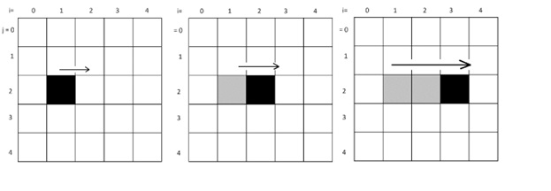
Consider a pixel at some location specified by coordinates (i,j). If it is ‘walking’ to the right, we get the situation seen below. The line will end up being horizontal, starting at (i,j), and proceeding to (i+1,j), (i+2,j) and so on.
A line can be straight or curved. A straight line can have any orientation or direction, and this is often indicated as an angle. It is a set of pixels where the next pixel is a fixed direction from the last one. A curve is more difficult to define and draw, but essentially does not have that property. All other types of lines are just variations of these two. Jagged lines, for example, are really just collections of regular lines of different angles joined end to end. Broken lines are straight lines with a common direction and a fixed sized gap between them.

vline (100, 100, 200)
drawPixel(x, y0)
drawPixel(x, y1)
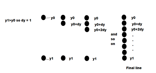
y = y0             // Starting Y coordinate
d = y1 – y0        // Number of pixels between y0 and y1
if d>0 let dy=1    // Line goes DOWN from y0
if d<0 let dy=-1   // Line goes UP from y0
y = y + dy         // Next pixel from y
drawPixel (x, y)   // Set this pixel to black
y = y + dy         // Next pixel
   . . .           // repeat the process
The algorithm is a description that could be followed by a non-programmer. It is not precise enough to be a computer program, though. The names x, y, y0, and y1 are variables, and in a program would need to be given a type in a declaration. What kind of variables are they? The sentence “repeat again from step 6 until y=y1” is something that a computer would have trouble with. Loops in a language have a specific syntax. The if is also something that each language implements in a specific syntax.
The code and algorithm for this is:
// Code:  code vline.pde                          Algorithm: vline – Draw a vertical line from (100, 100) to (100, 200)
int dy, y, y0=100, y1=200, x=100;                 The operation drawPixel(x, y) sets the pixel at (x,y) to black.
                                                    It’s really just set(x,y,color(0)
                                                  dy is the change in y on each pixel.
                                                  Y is the current vertical pixel position being drawn.
                                                  Y0 is the starting vertical position.
                                                  Y1 is the end vertical position.
                                                  X is the horizontal position.
size (300, 300);                                  Set the drawing area to 300x300 pixels

dy = y1-y0;                                       Distance between 200 and 100 (=100)
                                                  In this example y1-y0 is positive, meaning we are drawing down.
if (dy > 0) dy = 1;                               This tests to see if we go down or up from y0.
 else dy = -1;
for (y=y0; y != y1; y = y + dy)                   Set pixels to black starting at y0 and moving one pixel at a time to y1.
    drawPixel (x, y);

Changing y0 and y1 will change the start and end pixels for the line.
The syntax of the if and the for statements in Processing, the language we’re using here, can be found in Appendix I. The figure below shows how consecutive pixels are set in this method. Horizontal lines are drawn in an analogous way, this time fixing the y value and drawing between x0 and x1.
Algorithms for drawing general straight lines, which is to say between any two points P0 and P1, use some mathematics that should be vaguely familiar. It’s basically high school level, but for some it may have been some years since we looked at it. We will be setting pixels between the points (x0,y0) and (x1, y1) as before, but the orientation is arbitrary. The equation of a line is a mathematical relationship that tells us when a point lies on a line: if the equation is true (left side = right side) for some value of x and y, then (x,y) is on the line. Mathematically, a straight line is a set of points (which we can think of as pixels) that satisfy (I.E. result in a value of 0) an equation that defines a line. One such equation is:
The other commonly used equation for a line is the slope-intercept form, which is (of course) a variation of the two-point equation. Let’s let:
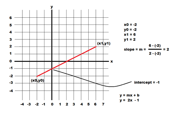
We have these two variations of the equation of a line, where one requires a slope and intercept and the other requires two points. In mathematics, there is a value x between any two values x0 and x1, and this is what makes mathematical lines continuous. In an image this is not true, and coordinates x and y are integers. If x1 = x0+1, there can be no value between x0 and x1, and this makes these pixel coordinate discrete.
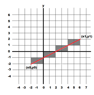
Drawing a line in a computer program usually means specifying the endpoints of the line and setting the pixels between them, so the two-point version could be the most useful. We need to draw the pixels where the (x,y) coordinates satisfy the equation. A problem is that it will rarely happen exactly on a raster grid, because the coordinates have to be integers, but the solution to the equation might not be. On a raster grid like a computer screen we select the pixels that are nearest to being actually on the line rather than a perfect solution. The lines will be a bit jagged, but at high enough resolution the line will look fine. For the line in the above figure the pixels that will be set are the grey ones in the illustration below.
Code: file dumb.pde                       Algorithm: dumb - Draw a general line

void dumb (int x0, int y0,                This syntax (See appendix I) defines an operation named
           int x1, int y1)                dumb that draws a line between (x0,y0) and (x1,y1).
{

                                          Define variables that we’ll need for this calculation.
float z, zz;
int a, b, c, d;
float m, bb=0;

a = (int)min(x0,x1);                      Range of x values is a .. b.
b = (int)max(x0,x1);
c = (int)min(y0,y1);                      Range of y values is c .. d
d = (int)max(y0,y1);

if (abs(x0-x1) > 0)                       Is the slope of this line defined (not infinite)?
{                                         If so, the slope m is The change in y divided by the change in x.
  m = ((float)(y0-y1)
       /(float)(x0-x1));
  bb = y0 - m*x0;
}
else
  m = 1000;                               Vertical. The slope is infinte. Just make it really large = 1000.
                                          There is no intercept with a vertical line.
for (int i=a; i<=b; i+=1)                 Examine all pixels (i,j) where x is between a and b and y is between
  for (int j=c; j<=d; j+=1)               c and d.
  {
    if (m > 900) zz = abs(i-x0);          If line is vertical and (i,j)is near the line then set pixel (i,j).
       else
     zz = abs((m*i)+bb-j);                If line not vertical then compute m*i+b-j.
    if (zz <= 1)
       set (i, j, color(0));              If smaller than 1 then set pixel (i,j) to black.
    }
}
We are allowing the distance between a pixel and the line to be 1 at most, which is what we would get if we rounded to the nearest integer. If the value is increased, the thickness of the line drawn increases too, as pixels more distant from the mathematical line are included. This one is not a very good example of a line generation algorithm. It’s pretty slow because it examines far too many pixels. The method used by most software to draw a line is a digital differential analyzer (DDA), and while the idea is pretty simple, the algebra can get complex.
The problem is: draw a line on a raster grid between (x1,y1) and (x2, y2). Start by setting the pixel (x1, y1).
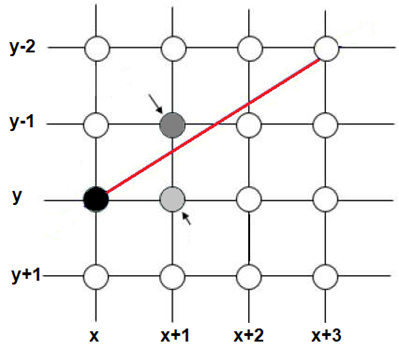
We can see a simple DDA below, where the line is drawn from (x, y) to (x+3, y-2) in screen coordinates. If we set
(x,y) the next pixel has to be either (x+1,y) or (x+1,y-1) – the actual line will pass between those locations. In
deciding which pixel to set we ask which of these pixels is closest to the actual line; that is, the line represented
by the equation. Visually, that would appear to be (x+1, y+1), so we set that pixel. Now look at the next pixel,
which is at (x+2,y-1) or (x+2,y-2). The pixel nearest to the line is (x+2,y-1), so we set that pixel, and so on.
The details of the algorithm specify which coordinate to increment, based on the line endpoints, and how to compute the distance (we use the line equation). However, this very accurately and quickly sets the pixels that belong to any line as specific by two points having integer coordinates. This is known as Bresenham’s algorithm to computer programmers, and tis also is implemented by the function line(), which is built into the Processing language.
There are many ways to draw a dashed line, and an easy one is to keep a count of how many pixels we have drawn; when a number indicating the length of a dash is reached, we set a flag to turn off drawing. This flag is true at the beginning of the line.
Each time a pixel is drawn (i.e. black) we count it, and when the count exceeds the number of pixels in a dash then set the drawing flag to false, and reset the count.
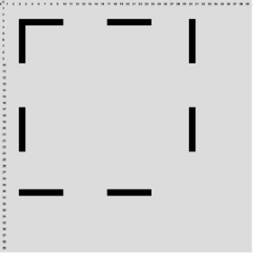
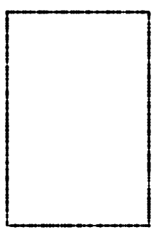
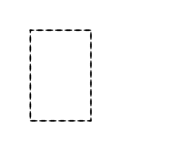
This method can, unfortunately, sometimes not draw the end pixels of a line if the final stage is one with drawing turned off. Consider drawing a square as four (dumb) lines:
  a = 3; b = 3; c = 30; d = 30
  dumb (a, b, c, b)
  dumb (c, b, c, d)
  dumb (c, d, a, d)
  dumb (a, d, a, b)
If we’re not careful there could be gaps at the end of the lines, and the square could look like the one here:
Code: file dumbdash.pde                  Algorithm: dumbdash - draw a dashed line
void dumbDash (int x0, int y0,
             int x1, int y1, int L0)
{

  float m, bb=0, z;                      Define slope, intercept, and other variables we need:
  float L, lox;                          L is the length of the line.
                                         lox is number of dashes
                                         L0 is the length of a dash
  int pcount = 0;

  boolean on = true;                     on = true is we are drawing, =false otherwise
  int a, b, c, d;

  L = dist (x0, y0, x1, y1);
  lox = (L/(2*L0));
  lox = lox - floor(lox);                NOW lox is number of partial dashes

  if (lox > 0.5) pcount = L0/2;          If lox>0.5 then there will be a
  else pcount = 0;                       gap, so start counting pixels half way through instead of at 0.

  a = (int)min(x0,x1);                   X extent of the line is a..b
  b = (int)max(x0,x1);
  c = (int)min(y0,y1);                   Y extent of line is c..d
  d = (int)max(y0,y1);

  if (abs(x0-x1) > 0)
  {
    m = (float)(y0-y1)/
        (float)(x0-x1);
    bb = y0 - m*x0;
  }
  else
    m = 1000;                           Vertical line has slope= m= 1000

  for (int i=a; i<=b; i+=1)             Examine all pixels (i,j) where x
  {                                     is between a and b and y is
    for (int j=c; j<=d; j+=1)           between c and d.
    {
      if (m >= 1000) z = abs(i-x0);     If line is vertical and (i,j) is near the line
                                         then set pixel (i,j).
       else z = abs((m*i)+bb-j);        If line not vertical then compute m*i+b-j. If smaller than 1 then:
      if (abs(z) <= 1)                  set pixel (x, y) to black if
      {
        if (on)                         drawing is turned on.
          drawPixel (i,j);
        pcount= pcount + 1              count drawn pixels.
        if (pcount >= L0)               If count is >= than the size of a dash, reset the count and
        {
          on = !on;                     turn drawing on if it’s off and off if it’s on.
          pcount = 0;
        }
      }
    }
  }
}
We could define a thick line as any line that is more than one pixel wide. The easy way to draw such a line is to draw
larger circles at each pixel on the line: change the code circle(i, j, 1) to circle(i, j, 5), for example, making the line 5 pixels thick. In the code we have been writing the function drawpixel() or set(i,j,color(0)) sets a pixel black, so we could simply modify this so that it would draw an circle of size t where t was the desired line thickness in pixels.
void drawPixel(int x, int y, int t)
{
  noStroke();
  fill (0);
  circle (x, y, t);
}
In fact, when using languages like Processing we can have multiple functions with the same name that depend on the number of type of the parameters, so both drawPixel(x,y) and drawPixel(x,y,t) can exist at the same time. The function
void lineThick(int x0, int y0, int x1, int y1, int thickness)
will draw thick lines in this way.
This is confusing, so look at THIS, where we define the parameters of such a line.
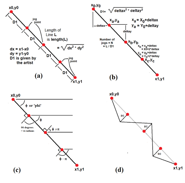
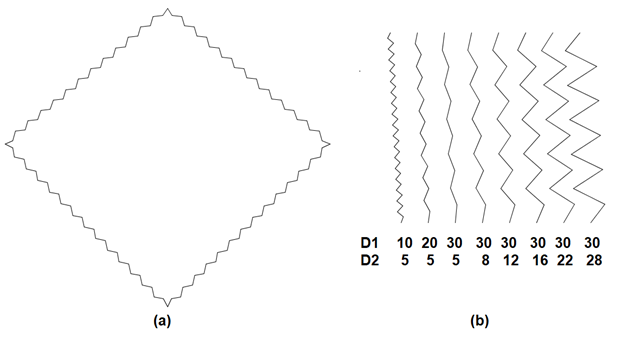
  x = x0; y = y0;               // Start point
  L = dist(x0, y0, x1,y1);      // Length of the line
  dx = x1-x0;                   // Total change in X
  dy = y1-y0;                   // Total change in Y
  N = (int)(L/d1);              // Number of jogs
  deltax = dx/N;                // X distance between jogs
  deltay = dy/N;                // Y distance between jogs
The first jog point is at (x0+deltax, y0+deltay), the second is at (x0+2*deltax, y0+2*deltay), and so on. At each jog point we construct a line (but do not draw it) through that point at 90 degrees (perpendicular) to the line L. The we find a point that is distance D2 from L along this perpendicular, where the artist has specified the value for D2 as the height of the jog. The angle the line L makes with the X axis is &phi =atan2(y1-y0, x1-x0), the inverse tangent function (If your trigonometry has been forgotten, then you’ll have to trust me). The perpendicular line to this has angle φ+90 degrees degrees or φ+π radians, an angle we’ll call γ).
  phi = (atan2(y1-y0, x1-x0));  // Angle of the line
  gamma = phi + (PI/2);         // Perpendicular
Of course, the angle φ-90 degrees is also perpendicular to L and indicates the other side of the line. Now we can begin drawing the jagged line, starting at xb=x0 and yb=y0. There are N jogs, so for each jog:
// For each step, find the point on the line and the one 90
// degrees from it distance d2.
  xb = x0;
  yb = y0;
  for (int i=1; i
Find the coordinates of the next jog point:
x = x0+i*deltax;
y = y0+i*deltay;
Determine the angle of the perpendicular line:
zeta = phi + sign*(PI/2);Sign will be +1 or -1, as we’ll see. Now find the point that is distance D2 from the jog point and that lies on this perpendicular. We need a bit of the most basic trigonometry for this:
dx = cos(zeta)*d2;
dy = sin(zeta)*d2;
xa = x+dx;
ya = y+dy;
The point (xa,ya) is the point we need. Now draw a line from the previous drawn point to this one:
line (xb, yb, xa, ya);The end of this line will be the beginning of the next:
xb = xa;
yb = ya;
Change the sign. This will result in the perpendicular points being on opposite sides of the line, making the jagged shape.
   sign = -sign;
}
And finally complete the line L, since it is unlikely that the final jog will end exactly on (x1,y1):
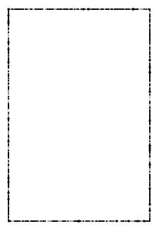
line (xb, yb, x1, y1);As an example, the figure below shows a rectangle drawn using jagged lines having D1=15 and D2=5, and also the results obtained by varying those parameters.
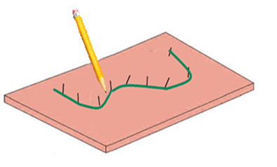
Let’s stay with the pencil example. How can we draw a line as if it we drawn using a pencil? Here’s a thought: create a pencil texture –scan an image created using a real pencil to shade an area on paper – and then use pixels from that image instead of using a specific line color. Take a pencil and create a shaded area, the scan that image. This creates an image such as the 517x286 pixel image below:
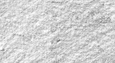
When we draw a line using this texture, we simply copy pixels from this image into the line as we draw it. If we are drawing a line from (100,100) to (400,300) we use a different version of the drawpixel function, one that sets pixels according to values it finds in the image, rather than to a fixed value like black. If we draw a pixel at (x,y), we use the pixel at (x,y) in the pencil texture image as the value. If that pixel is outside of the texture image we can simply map the pixel coordinates onto the texture using the mod operation, which is % in most programming languages. So if drawing a pixel at (1031, 853), we use the texture pixel at (1031%w, 853%h), where (w,h) are the maximum coordinates in the texture image.
Drawing a rectangle with upper left corner at (100,100) and lower right corner at (900, 600) means sampling pixels from the pencil image rather than setting them to black, and can be accomplished using:
void drawtpixel(int x, int y, int t)
{
  color p;

  for (int i=-t/2; i
The parameter t is the line thickness. This function copies pixel values from a texture image and draws them into a
t/2 by t/2 sized area in the target image. The function
void tLine(float x1, float y1, float x2, float y2, int t)
uses this function to draw the pixels, as illustrated below:
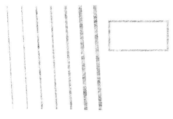
What is the desired thickness? How should it vary? That would be up to the artist, and should be simple to specify. SO: should the line thickness be random? Should it follow a predefined pattern? Should it depend on some other aspects of the artwork? To draw a line of variable thickness that is random, we call the function drawpixel(x,y,t) whenever we draw on of the pixels in the line, whichever line drawing method we’re using and specify the thickness value t using a random number. Like so, perhaps:
drawpixel (x,y,round(random(1,t)));
This should draw a line having a completely random thickness of between 1 and t pixels:
// Random
int thick(int t)
{
  float x, r;

  x = random (1, t);
  if (x<=0) x = 1;
  else if (x>t) x = t;
  return (int)x;
}
This should draw a line having a regular sine/cosine variation in thickness:
//Cosine
float _z = 0;
int thick(int t)
{
  float x, r;
  x = abs(cos(_z)) * t;
  _z += 0.1;
  if (x<=0) x = 1;
  else if (x>t) x = t;
  return (int)x;
}
// Random Average
Float prev = 2;
int thickavg(int t)
{
  float x, r;

  r = random (-1, 1);
  x = t/2 + r;
  x = (x + prev)/2;

  if (x<=0) x = 1;
  else if (x>t) x = t;
  prev = x;
  return (int)x;
}
arc (a, b, c, d, start, stop)where: (a,b) are the coordinates of the center of the ellipse
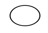
Let’s start explaining this rather hard to characterize shape by beginning with the problem of drawing an ellipse as four arcs. Consider the ellipse:
ellipse (300, 200, 100, 80); |
|
stroke (128); arc (300, 200, 90, 80, radians(0), radians(90)); |
|
arc (300, 200, 90, 80, radians(90), radians(180)); |

|
arc (300,200, 90,80, radians(180), radians(270)); |

|
arc(300, 200, 90, 80, radians(270), radians(360)); |

|
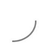
We know the equation of an ellipse, so for any given x value the y values of pixels on the ellipse are known.
Given the point (xc, yc) at the center of the ellipse, we wish to know what the pixel coordinates are at an
angle of θ degrees from that point. A way to picture this is to draw a line from (xc, yc) having an angle θ
and see where it intersects the ellipse.
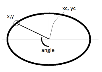
float[] startPoint (float xc, float yc, float w, float h, float angle)where: (xc,yc) is the center of the ellipse.
pts = startPoint (x, y, w, h, a);and the point (pts[0], pts[1]) is the location we are looking for. (The variable PTS is an array - see the appendix). Now what? We want to continue the curve from that point in some direction to somewhere else. As a practical example, let’s use a section of the vase. To top left curve in the vase was drawn by:
arc (65, 75, 33, 64, radians(295), radians(360+65));The parameters of the next section were found using graph paper.
arc (80,190, 87,172, radians(135), radians(258));
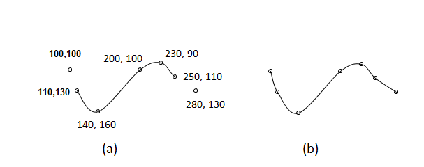
  beginShape();
    curveVertex(100, 100);
    curveVertex(110, 130);
    curveVertex(140, 160);
    curveVertex(200, 100);
    curveVertex(230, 90);
    curveVertex(250, 110);
    curveVertex(280, 130);
  endShape();
The beginShape() says to begin drawing a shape made of points. Each curveVertex() specifies
one point to be drawn that is a part of the curve, in the order they appear on the curve.
The process stops when endShape() is seen. We could expect this code to draw a smooth curve between
7 points: not quite. In order to draw a curve we need to know something about the shape of the curve at every
point, and we get that information from the preceding and successive points on the curve. The first point
does not have a preceding point, though, and can be used only to provide shape context for the second point.
A similar situation applies at the final point, as in the figure below.
  beginShape();
    curveVertex(100, 100);
    curveVertex(100, 100);
    curveVertex(110, 130);
    curveVertex(140, 160);
    curveVertex(200, 100);
    curveVertex(230, 90);
    curveVertex(250, 110);
    curveVertex();
    curveVertex(280, 130);
endShape();
So to connect a set of points using a spline, we simply place them in sequence in curveVertex() calls
between a startCurve() and endCurve(), duplicating the first and last pixels. We can draw any
set of points this way. We can adjust the shape of the start and end by adjusting those coordinates until the
shape looks OK, as in figure b above.
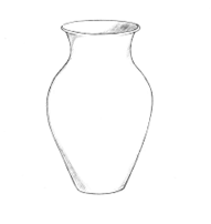
At this point, note that the vase is not symmetrical. It probably should be.
A solution is to divide it in two vertically and choose which half to draw. When this is complete
simply redo the same curves as a mirror image.
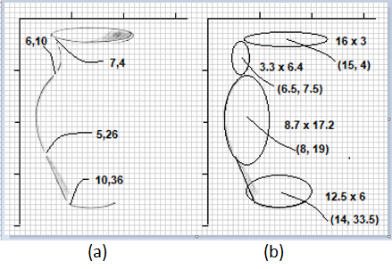
Creating the grid allows us to determine coordinate values, at least approximately.
For this example we require the dimensions of each ellipse and the coordinates of the
center. With the first guess a preliminary view can be created by just drawing the ellipses and the lines.
ellipse (150,40, 160,30);
ellipse (65,75, 33,64); ellipse (80,190, 87,172);
ellipse (140,335, 125,60);
line (55, 270, 90, 350);
This is a fair approximation for a first guess. Now we have to estimate the angles from which to subtend the arcs and then draw those instead of ellipses. The first estimate can be eyeballed or measured with a protractor.
The first four parameters of the call to arc will be the same as the ones passed to ellipse:
the center coordinates and the size. The start and end angles are estimated as:
stroke (255, 0, 0);
arc (65,75, 33,64, radians(295),radians(405));
arc (80,190, 87,172, radians(110), radians(250));
arc (140,335, 125,60, radians(45), radians(135));
line (55, 270, 90, 350);
Because the arcs must be drawn in a clockwise fashion, the first curve runs from 295 degrees (a little past the top right) to 405 degrees, which is 360+45 or simply 45 degrees. The line coordinates have been adjusted a little as well.
We’re not quite there yet. There are some small adjustments to be made to close the gaps and smooth things. The first two curves seem OK. The third one fails to meet the second correctly, so a good idea would be to adjust the angles. Extending the ends of both curves works pretty well, and the height of the third is increased just a bit so that they meet relatively smoothly.
The third curve extends too far at its beginning and is shortened by increasing the start angle.
The line must be lengthened so as to meet the new start point.
Finally, when this is done the bottom of the vase does not quite meet the straight line.
The line end coordinate is changed slightly and the bottom curve is moved a pixel to the left.
The new code is:
    ellipse (150,40, 160,30);
    arc (65,75, 33,64,
    radians(295), radians(360+65));
    arc (80,190, 87,172,
    radians(135), radians(258));
    arc (149,335, 150,70,
    radians(45), radians(135));
    line (49, 250, 93, 358);
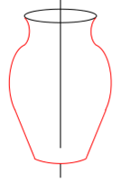
The vertical line in the figure is the axis of symmetry. The vase should look the same on both sides of this line. It is not obvious how to do this. The vertical line is at X=150, so it would be possible to copy the individual pixels from the left side to the same distance from the symmetry axis on the right. This method works but is not interesting. Isn’t it better to know how to manipulate the curves geometrically?
So, first consider the arc near the mouth of the vase. Its location is (65, 75) and the vertical axis is x=150, so the center coordinates of the symmetric version of the arc would simply be (150-65+150, 75) or (235, 150). The size will remain the same. The angles also follow a symmetry that is simple to compute once it is understood. Simply put, angles can be express as negative or positive. -45 degrees is simply 360+ (-45) or 315 degrees. The -45 representation tells us how far in a counter clockwise direction the same amount of rotation 45 degrees is. Each angle on the left should be replaced by the same, negative, angle drawn on the right of the axis of symmetry. THEN it should be rotated by 180 degrees. The operation that returns the angle on the right given the angle on the left (or vice versa) is: a = -a+180.
Finally, the start and stop angles need to be swapped. If they are in clockwise order on the left,
then they will be counter-clockwise on the right. The corresponding pixels are specified by:
arc (300-65, 75, 33, 64, radians(-425+180), radians(295+180));
After an adjustment of a few pixels at the bottom, the image is in pretty good shape.
Of course, this has been a highly interactive process, with manual adjustments taking place
at many stages. That’s because this shape does not have a specific mathematical description.
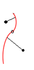
One of the problems that needs to be solved when using curves is how to continue from the end of
one curve directly to the next and how to create a curve that connects two or more points.
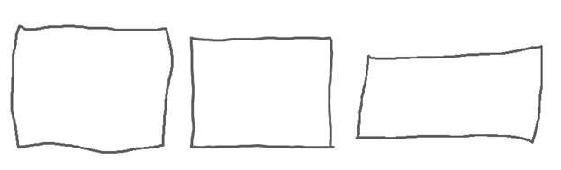
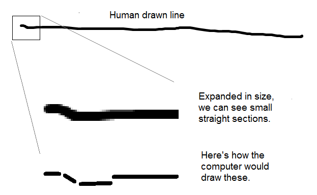
Two were drawn freehand using Paint and a mouse on a PC and one was drawn by a Processing program that was written for this book. Which is which? How is a human drawn line different from a perfectly straight line? We are about to embark of a rather complex method that involves both artistic vision and algorithms.
The rectangle in the middle was drawn by a computer. The process for designing the method is not a long and tedious one: we’ll measure some lines drawn by humans and try to do the same. A human can’t connect two points that are far apart with a perfect line, but perhaps can connect nearer points. If true, this means that a long human line is a set of smaller quite straight lines. How small? We don’t know, but could guess and then see how it looks, then guess again. And we’ll use random numbers.
Let’s say that a variable named lthresh will hold a number that indicates how long a typical straight
line is that is drawn by a person. Any line to be drawn will be broken into smaller sections that are about
this long, but in fact have random lengths averaging this value. Let’s draw a line from (x0,y0) to (x1,y1).
The length of this line is
√((x1-x0)2+(y1-y0)2)
which is called Euclidean distance) as we learned in high school math, or in Processing it would be:
llength = sqrt ( (x1-x0)*(x1-x0) + (y1-y0)*(y1-y0));
If this is less than lthresh then we’ll simply draw it., otherwise split the line into two parts:
one will be a random length larger than lthresh and the other part will be the rest of the line.
The rest of the line will be broken into smaller length for drawing later. We know this because of looking
at actual human drawn lines.
newLength = random (lthresh, 2*lthresh);How do we split up a line? Consider the line below:
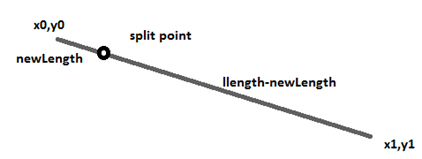
The problem is that we need the actual coordinates of the split point, because that’s how Processing
draws lines: from one known point to another. How can we find those coordinates? We do know the ratio
of the lengths of the short part to the long part and to the entire length, but that’s all. It happens
to be good enough. The fraction of the whole line that we’re drawing this time is newlength/llength.
This should also be the fraction of the vertical and horizontal parts of the line we’re drawing.
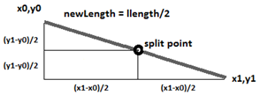
So, the X coordinate of the split point should be at a point newlength/llength * (x1-x0) from the
start point x0, and ditto for the Y coordinate. Or:
nx = xx+(int)((xe-xx) * fraction);
ny = yy+(int)((ye-yy) * fraction);
If the split point were in the middle of the line then the geometry would be like this:
We need to break here to examine likelihoods a bit. When we toss a coin we expect it land with either the heads side up or the tails side up. We expect that the chance of each outcome will be the same, which we call 50-50. As a probability this would be 0.5. Something that will never occur has a probability of 0.0, and something that must occur has a probability of 1.0. Sometimes a weather forecaster will say “The probability of rain today is 25%”, meaning that there is a 0.25 (or 25/100) chance of rain.
The variable vpct represents probability that the line endpoint will change in one of the
four possible ways: increase nx, decrease nx, increase ny, or decrease ny.
The value of random(1) is a random number between 0 and 1, so, if random(1) < vpct then add 1 to nx.
In fact:
if (random(1) < vpct) nx = nx + 1;
      else if (random(1) < vpct) nx = nx - 1;
  if (random(1) < vpct) ny = ny + 1;
      else if (random(1) < vpct) ny = ny - 1;
These are the four ways the endpoint can change, and this code makes it happen. The value of nx can either get bigger or smaller, as can ny. Now we draw the line from (x0,y0) to (nx,xy).
This is not the end, because we’ve only drawn one small section of the line. The remainder of the line is
from (nx,ny) to (x1,y1). Next we break that part of the line into two pieces as was done before, find a
new (nx,ny), draw that piece, and continue until the end of the line is reached.
Code: File human.pde’ Algorithm: human – Draw a line that looks like a human might have drawn it.
// Draw a line from (x0,y0) to (x1,y1)
float len, newLength, fraction; The variable len is the length of the line.
int xx, yy, nx, ny; (xx,yy) will be the pixel we are drawing from. Start at (x0,y0).
len = sqrt ( (x1-x0)*(x1-x0) +
(y1-y0)*(y1-y0));
xx = x0; yy = y0;
while (xx
The parameters that will make these lines change to be more or less like human ones are vpct, and lthresh. As vpct gets smaller the likelihood of each component of the line begin changed gets smaller, and so the line becomes straighter. As lthresh gets larger the length of the line a human can draw gets longer, and so the line appears straighter. If lthresh becomes very large or vpct gets very small then the lines become perfectly straight. If lthresh gets too small or vpct gets too close to 1.0 then chaos could result.
This happens to be a much more difficult problem than drawing them. A pixel may not belong to any line.
A pixel may be at the intersection of many lines, and so belong to all of them. There are a great many
pixels in a typical image, and it could be very time consuming to try to find all of the lines that
might pass through all of the pixels. One advantage we had when drawing the lines in the first place is knowing where the endpoints were; in an image we don’t know that. And finally, images acquired in the real world (photos, for example) contain lines from the real world and not from the discrete world of the computer. A DDA did not create those lines.
How can we possibly solve this problem? We can use mathematical trickery or brute force.
The Chord Property
Pixels that form a line possess many geometric properties, and one is the chord property. Assume that there is a collection of points that we will call S. The collection S has the chord property if for any points p and q in S, the line segment between p and q there is a lattice point (i,j) so that max(|i-x|, |j-y|) is smaller than 1. Wow, that seems a brain teaser, but it’s simpler to see from Figure 2.37. The lattice points are just grid points or integer coordinates. The figure shows a straight line and the pixels (lattice points with black colored circles) that belong to it. Any line drawn between two points that belong to that line must lie completely within the green boxes. That’s what the chord property says.
Here's an important thing to know: any collection (set) of pixels S that has the chord property is a straight line segment. So what we can do is gather pixels into a collection and keep testing the chord property, and so long as it holds the pixels belong to a line. When it fails, remove those pixels from the image and save them as a line segment. In fact, simply save the two end points, because that’s all we really need.
Something that we can do to make things faster and easier is to start with some black pixel in the image and add black pixels that are connected to it and have the chord property, one at a time. When the chord property fails we have a connected set of pixels that form a line.
Wait, connected? What’s that?
We can define connected easily enough – it simply means next to each other, or adjacent. We can define pixels to be connected in two ways – they can be 4-connected or 8-connected. They are 4-connected if they are adjacent in the same row or column. If there is a pixel at location (i,j) then the pixels at (i-1,j), (i+1,j), (i, j-1) and (i,j+1) are 4-adjacent, and if they are the right color (black) then they are said to be 4-connected, because there are 4 possible pixels next to it. Any pixel has 8 pixels surrounding it, and those are the 8-adjacent pixels: the previous four (i-1,j), (i+1,j), (i, j-1) and (i,j+1), as well as (i-1,j-1), (i-1,j+1), (i+1,j-1) and (i+1, j+1). Adjacent pixels are next to each other.
So, we define pixels to be 4-connected if there is a set of 4-adjacent black pixels connecting them, and 8-connected if there is a set of 8-adjacent pixels connecting them. We usually think of lines as 8-connected, but that’s not required.
Now here’s how we identify, or extract if we like, lines from an image. First find a black pixel – we assume lines consist of black pixels. This will be our starting pixel. This is pretty simple, but it also does one other thing – it adds this first pixel to the set we called S, and changes the pixel’s value in the image to white so we don’t use it again.
Given a black starting pixel, the next step is to find a black 8-neighbor. We look at all horizontal, vertical, and diagonal neighbor pixels. There could be many of these – which one do we want? The one that, when added to S, gives the smallest chord value. Of course it has to be less than 1 to be acceptable, but it could have values between 1 and 0. Smaller is better. We will have to look at all 8 adjacent pixels and, if it is black, determine what the chord property value is, remembering only the smallest. Let the black neighbor with the smallest chord value be the pixel (bi,bj) and the chord value is bv. If bv<1 then add (bi,bj) to S.
Now we have added a second point (maybe) to the set. We should carry on from here and try to find another, which will be adjacent to (bi,bj), etc etc. So simply set ca =bi and cb=bj and do it all again. In other words, put all of the code in a while loop. It will exit from the function, and hence from the loops, when bv>1, from the code above. When that happens the set S will contain the coordinates of all of the pixels in the line, if there are any. We can draw it or save it, set N=0 and start again, searching for another start pixel.
The functions we have are:
initialize (Pimage im) // Find a start pixel. Save it in S.
addToS(im,bi,bj) // Add another pixel to S and set it WHITE.
vectorize (PImage im) // Find another line in the image im.
float chord(ni,nj) // Check to see if we can add (ni,nj) to S.
// Return the chord value, 10000 if not.
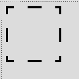
Testing this extensively takes a long time and lots of data. A simple test could be an image containing a small square, though. In Figure out.png, the original image is on the left. The lines extracted by the program are on the right. This seems pretty good, but this is a simple image: the lines ae perfect (drawn by code) and are of thickness 1. Things get trickier when we use real, captured images.
In case it has not been obvious, the point here is to find lines in images so we can create a sketch, or a new rendering of some sort involving lines. When a human artist makes a pencil drawing, they usually outline the shapes they see, and then progress to shading. This means that they must be able to transform a complex multi-level image into basic lines. One of the important issues in this chapter is to show how complex this task is, and to give some ideas on how to do it using a computer. As well will see, this specific algorithm is far from perfect, but gives a good start.
The chord function, which is basic to this vectorization process, has been left for last to increase suspense. Here it is:
Code: File chord.pde’
float chord (int ni, int nj)
{
float dx, dy, slope=0, b=0;
float dsum,xp,yp,d;
int i;
dx = (float)(getSx(0)-ni);
dy = (float)(getSy(0)-nj
dsum = 0.0;
for (i=1; i
Straight lines, if they are digital straight lines, can be identified in an image.
What about curves? In a digital image we know which pixels are black and which are white,
and we collect them into sequences of connected pixels that could be part of a curve. Then we can draw them again using a spline, assuming that they do form a curve, to recreate the original curve. A measure of how well this process has worked is a measure of how similar the original image is to the one that is drawn.
One algorithm for identifying a sequence of pixels that belongs to a curve is the chain coding algorithm.
We trace pixels along a curve one at a time, starting at some obvious place: either a pixel that is connected
to only one other pixel, or a pixel that is connected to two pixels on opposites sides. The method uses the
neighbors of each pixel in a line or curve, and steps through them while recording the direction that
was used in each step. We obviously must use the same directions all the time. Each pixel has 8
neighbors, so there are eight directions, and they are numbered as seen in Figure 2.41a.
There’s no reason for this numbering except that it is commonly used by others. Figure 2.41b
shows how this set of black pixels would be traced.
The essential chain coding algorithm is :
Drawing from a chain code means simply beginning at any pixel P, set it to black, move in the direction of
the first code value to find the next pixel, set it to black, and so on until all code values are used.
Let’s see how that works for curve extraction. Figure 2.42 shows a line drawing (left) and the chain code
reconstruction (right), which has 39 sections. That means that each section is a distinct curve that can
be manipulated independently from the other parts.
A thick line is one that is more than a single pixel wide. To be a line, it must also be much longer
than it is thick. Figure 2.43a shows and object and the corresponding thin line, also called the skeleton.
Identifying the pixels that form the skeleton is not as easy as it may appear. A skeletal pixel is
equidistant from the opposite sides of the shape, and opposite sides can be a tricky business to
compute. The skeleton will be continuous, having no gaps. And it will be one pixel thick.
There is no known perfect method for finding skeletal pixels, but methods for doing so – called thinning
algorithms – all of them strip pixels from the outline one layer at a time, making certain that the skeleton
remains a single continuous set of pixels. The pixels having distance 1 from the background are removed
first, then those with distance 2, and so on, never removing any pixel that would break the skeleton into
two parts. Figure 2.44b shows these distances are grey values – the dark object pixels are nearest to the
background, and the light ones are farthest away. This image is called the distance transform of the original
object. It’s not the skeleton, but it's a start.
The details of any good thinning algorithm are a bit specialized and ugly. There are known problems that
have special cases that are handled using specific functions. Ugh. A thinning method that seems pretty good
generally is given as ALGZHANGSUEN for everyone to use. It assumes that the input image consists only of
black or white pixels, and yields a connected skeleton of the objects in the image. An example of input to
and output from this program is in Figure 2.30.
Imagine that we have an image of a pencil or ink drawing, such as that shown in Figure 2.45. This is an
unusual starting point, but in later chapters we’ll discuss how to convert an arbitrary photographic
image into such a thing. It was created from a human artwork (an india ink painting by the author) .
Here are a few simple processes we can apply to it that can produce interesting visual effects.
1. Find the outline of the image. Based on the methods seen so far, this is not difficult: keep all black pixels that have a non-black neighbor, and set the resut to white. More will be said on this in the next chapter. The result is Figure 2.46a.
2. We could now vectorize the outline and draw it as vectors. Since we have endpoint coordinates, we can draw the vectors at difference sizes (scales). For example, to draw it at ½ the original size, simple multiply all of the endpoint coordinates by ½ before drawing them. Figure 2.46b shows the result of this for 20 repetitions of scaling and drawing using a 5% reduction (multiply by 0.95) each time.
3. Using the scaling idea, we can scale in the X and Y axes differently (Figure 3.46c). (Some of the ‘background’ lines were make lighter using Paint)
Depending on the image we use, there are many things we could try. An advantage of generative art is that we can make many changes in the method very quickly and keep the ones we like the most.
We can also use other digital or traditional tools applied to a generative result. The image in Figure 2.47 is the result of coloring the background of the 2.46a image using Paint, and than drawing the extracted edges over top of that image. This could have been done with programs and algorithms without using Paint, as we’ll see in the next chapters. We could use lines of varying thickness, textured lines, or simulated human drawn lines. Or thousands of other variations
References
Adrrian Bowyer and John Woorwark (1983) A Progremmer’s Geometry, Butterworth-Heinemann Ltd; Reprint edition. ISBN-13 978-0408012423
J. E. Bresenham (1965). Algorithm for computer control of a digital plotter, IBM Systems Journal. 4 (1): 25–30. doi:10.1147/sj.41.0025
Edwin Catmull, Raphael Rom, (1974). A class of local interpolating splines. In Barnhill, Robert E.; Riesenfeld, Richard F. (eds.). Computer Aided Geometric Design. pp. 317–326. doi:10.1016/B978-0-12-079050-0.50020-5.
James D. Foley, Andries van Dam, Steven K. Feiner, and John F. Hughes (2013) Computer Graphics: Principles and Practice (3rd Edition). Addison-Wesley Professional. ISBN-13 978-0321399526
Freeman, Herbert (June 1961). On the Encoding of Arbitrary Geometric Configurations. IRE Transactions on Electronic Computers. EC-10 (2): 260–268. doi:10.1109/TEC.1961.5219197
Lyche T, Manni C, Speleers H (2018). Foundations of spline theory: B-splines, spline approximation, and hierarchical refinement. In: Lyche T, Manni C, Speleers H (eds) Splines and PDEs: from approximation theory to numerical linear algebra, vol 2219 of Lecture notes in mathematics. Springer, Berlin
Marchand-Maillet S, Sharaiha YM (2000) Binary digital image processing — a discrete approach. Academic Press, Maryland
Isabella Meyer (2022). Paul Klee – Modernist, Colorist, Theorist, and Innovator(Updated February 10, 2024) https://artincontext.org/paul-klee/
James Parker (1988). Extracting vectors from raster images, Computers & Graphics, vol. 12, pp. 75-79.
James Parker (2022) Randomness in Generative Art: Drawing Like a Person, Academia Letters,https://api.semanticscholar.org/CorpusID:245939262
T. Y. Zhang and C. Y. Suen(1984) Fast Parallel Algorithm for Thinning Digital Patterns, Communications of the ACM, Volume 27 Number 3, March
Tools and Examples
arc - Examples of ellipse and arc. Extracting Curves From Pixels
	Choose a direction (clockwise or counter-clockwise). We chose counter-clockwise.
	Select a starting pixel in the image (In figure 2.41 it is the red pixel). If we wish to reproduce this curve in its original location then we have to save these coordinates.
	Choose a starting direction D to look for a neighbor. We choose 5, because we looked at the row above and the previous column already in our search for a start pixel, and found no black pixels.
	Is the neighbor in direction D black?
	If not:
5a. Select the next direction for D, which is D+1. If D=7, next is 0.
5b. If we have tried all eight neighbors, then go to step 7.
5c. Continue from step 4.
	If so:
6a.  Save the value D as the next element in the code.
6b. Continue from step 4.
	Quit
In the example of Figure 2.40b, the code will be “656670012324”, and would continue forever because
the curve ends where it begins. To prevent this, we set the pixels to white in step 6a.
Thick and Thin Lines (Again)
If an image consists of lines, the digitized version could have those lines represented as an arbitrary
thickness depending on the optics of the process. An original image with one-pixel thick lines could have
three-pixel thick lines in the captured version, for example, or vice versa. This could cause problems
when processing the image later. Also, sometimes we take a photograph and wish to make a line drawing
using existing boundaries and lines. Again, these might not be one pixel thick. We saw in a previous
section how to draw thick lines. If we have an image with thick lines in it, can we make them thinner?
To some degree, yes.
What Use Is This?
The utility of any individual algorithm is limited by the imagination of the personusing it. And artist
would rarely say to themsleves “How shall I use a thinning algorithm today?” and more than an electrician
would say “How shall I use my pliers today?”. These are tools to be used when the opportunity requires.
This is only chapter 2, and all we really know about formally are things to do with black and white pixels
and lines, so the choices are limited by that experience. On the other hand, lines are used by artists to
draw things. We might be able to do a simple drawing from a scene (image).
fig223 - Code that draws figure2.23 using splines
quorra.pde - Generative art example – drawing of Quorra
human - System for drawing human style lines
startPoint - Animation of ellipse/line intersection
vase - Drawing the vase example
Library – Code provided for you
bresenham - DDA line drawing
chain - Chain code extraction
ChainCurve - Chain code class
chord - Chord property vectorization
drawPixel - Draw one pixel
dump - Slow, obvious way to draw a line
dumbdash - Dashed lines
llibrary02 - Main program for testing
lineThick - Thick lines
newline - Line tracing
slopeint - Slope-intercept lines
startPoint
texture - Textured lines
thin - Line thinning
vAverage - Variable thickness lines, moving average
vCosine - Variable thickness lines, cosine based thickness
vNoise - Variable thickness lines, uses noise
vRandom - Variable thickness lines, random thickness
vline - Vertical line
zig - Zig-zag lines